Author: mike (Page 4 of 26)

Using IOKit to Detect Graphics Hardware

October 21, 2011 / mike / 6 Comments

After Seasonality Core 2 was released a couple of weeks ago, I received email from a few users reporting problems they were experiencing with the app. The common thread in all the problems was having a single graphics card (in this case, it was the nVidia 7300). When the application launched, there would be several graphics artifacts in the map view (which is now written in OpenGL), and even outside the Seasonality Core window. It really sounded like I was trying to use OpenGL to do something that wasn’t compatible with the nVidia 7300.

I’m still in the process of working around the problem, but I wanted to make sure that any work-around would not affect the other 99% of my users who don’t have this graphics card. So I set out to try and find a method of detecting which graphics cards are installed in a user’s Mac. You can use the system_profiler terminal command to do this:

system_profiler SPDisplaysDataType

But running an external process from within the app is slow, and it can be difficult to parse the data reliably. Plus, if the system_profiler command goes away, the application code won’t work. I continued looking…

Eventually, I found that I might be able to get this information from IOKit. If you run the command ioreg -l, you’ll get a lengthy tree of hardware present in your Mac. I’ve used IOKit in my code before, so I figured I would try to do that again. Here is the solution I came up with:

// Check the PCI devices for video cards. 
CFMutableDictionaryRef match_dictionary = IOServiceMatching("IOPCIDevice");

// Create a iterator to go through the found devices.
io_iterator_t entry_iterator;
if (IOServiceGetMatchingServices(kIOMasterPortDefault, 
                                 match_dictionary, 
                                 &entry_iterator) == kIOReturnSuccess) 
{
  // Actually iterate through the found devices.
  io_registry_entry_t serviceObject;
  while ((serviceObject = IOIteratorNext(entry_iterator))) {
    // Put this services object into a dictionary object.
    CFMutableDictionaryRef serviceDictionary;
    if (IORegistryEntryCreateCFProperties(serviceObject, 
                                          &serviceDictionary, 
                                          kCFAllocatorDefault, 
                                          kNilOptions) != kIOReturnSuccess) 
    {
      // Failed to create a service dictionary, release and go on.
      IOObjectRelease(serviceObject);
      continue;
    }
				    // If this is a GPU listing, it will have a "model" key
    // that points to a CFDataRef.
    const void *model = CFDictionaryGetValue(serviceDictionary, @"model");
    if (model != nil) {
      if (CFGetTypeID(model) == CFDataGetTypeID()) {
        // Create a string from the CFDataRef.
        NSString *s = [[NSString alloc] initWithData:(NSData *)model 
                                            encoding:NSASCIIStringEncoding];
        NSLog(@"Found GPU: %@", s);
        [s release];
      }
    }
		    // Release the dictionary created by IORegistryEntryCreateCFProperties.
    CFRelease(serviceDictionary);

    // Release the serviceObject returned by IOIteratorNext.
    IOObjectRelease(serviceObject);
  }

  // Release the entry_iterator created by IOServiceGetMatchingServices.
  IOObjectRelease(entry_iterator);
}

File Vault 2 on the 2011 MacBook Air

October 20, 2011 / mike / 0 Comments

I recently upgraded to a 2011 MacBook Air. With the new Sandy Bridge processors having encryption routines built-in, I decided to try out File Vault 2 on Lion to see what kind of performance impact it would have while accessing the disk. Here’s the configuration of my MacBook Air for reference:

11″ MacBook Air (Summer 2011)
1.8Ghz Core i7
256GB SSD (Samsung model)

First the baseline. Before enabling File Vault, I did a quick test of writing a 10GB file and then reading it back.

Blade:~ mike$ time dd if=/dev/zero of=test bs=1073741824 count=10 10+0 records in 10+0 records out 10737418240 bytes transferred in 41.938686 secs (256026577 bytes/sec) real 0m42.021s user 0m0.005s sys 0m6.827s Blade:~ mike$ time dd if=test of=/dev/null bs=1073741824 count=10 10+0 records in 10+0 records out 10737418240 bytes transferred in 37.969485 secs (282790726 bytes/sec) real 0m38.055s user 0m0.005s sys 0m5.069s

After enabling File Vault, the Mac restarts and it took about 50 minutes to finish the initial encryption. While the encoding was taking place I was seeing roughly 95-120MB/sec transfer rates (190-240MB/sec combined read/write bandwidth), and it averaged about 45-50% CPU usage (% of a single core) during the encoding process.

So what how was performance with encryption enabled? Check this out…

Blade:~ mike$ time dd if=/dev/zero of=test bs=1073741824 count=10 10+0 records in 10+0 records out 10737418240 bytes transferred in 45.342448 secs (236807202 bytes/sec)


real	0m45.418s

user	0m0.001s

sys	0m7.721s

Blade:~ mike$ time dd if=test of=/dev/null bs=1073741824 count=10

10+0 records in

10+0 records out

10737418240 bytes transferred in 40.052954 secs (268080558 bytes/sec)

real 0m40.133s user 0m0.001s sys 0m4.032s

So read operations take a 5.5% hit, and write operations are 8.1% slower with File Vault 2 enabled. That’s a performance penalty I can live with for the extra peace of mind of my data being secure while traveling. Even better is the amount of CPU used was about the same whether encryption was enabled or disabled.

Performance summary:

File Vault	Read		Write
	Bandwidth	CPU	Bandwidth	CPU
Disabled	269.69 MB/s	5.074s	244.16 MB/s	6.832s
Enabled	255.66 MB/s	4.033s	225.84 MB/s	7.722s

When the App Store thinks an app is installed when it really isn’t

October 5, 2011 / mike / 1 Comment

I was trying to figure out a problem where the Mac App Store incorrectly thought an application was installed on my Mac. For the life of me, I couldn’t figure out why it thought that app was installed when it wasn’t. I tried deleting caches, restarting the Mac, Spotlighting for all apps with that name, all to no avail.

It ended up the problem was from the LaunchServices database. The App Store checks LaunchServices to see which apps are installed. Apparently LaunchServices still had a record of an application bundle even though it had been deleted. Here’s how to use the Terminal to check and see which apps are in the LaunchServices database:

/System/Library/Frameworks/CoreServices.framework/\ Versions/A/Frameworks/LaunchServices.framework/Versions/\ A/Support/lsregister -dump

If you search through that verbose output and find an app that isn’t really there, you should rebuild the LaunchServices database. You can do that with the following command:

/System/Library/Frameworks/CoreServices.framework\ /Versions/A/Frameworks/LaunchServices.framework/Versions\ /A/Support/lsregister -kill -r -domain local -domain system -domain user

Hope this saves someone an hour or two of problem-solving…

Shrinking a Linux Software RAID Volume

August 17, 2011 / mike / 9 Comments

I upgrade the disks in my servers a lot, and often times this requires replacing 3-4 drives. Throwing the old drives out would be a huge waste, so I bring them back to my office and put them in a separate Linux file server with a ton of drive bays. I wrote about the fileserver previously.

In the file server, I configure the drives into multiple RAID 5 volumes. Right now, I have 3 RAID volumes, each with four drives. Yesterday, one of the disks in an older volume went bad. So right now I’m running 3 out of 4 drives in a RAID 5. No data loss yet, which is good. Since this is an older RAID volume, I’ve decided not to replace the failed drive. Instead, I’ll just shrink the RAID from 4 disks into 3 disks. It was quite a hassle to figure out how to do this by researching online, so I thought I would document the entire process here, step by step, to save other people some time in the future. It should go without saying that you should have a recent backup of everything on the volume you are about to change.

Make sure the old disk really is removed from the array. The device name shouldn’t show up in /proc/mdstat and mdadm –detail should say “removed”. If not, be sure you mdadm –fail and mdadm –remove the device from the array.

# cat /proc/mdstat
Personalities : [linear] [multipath] [raid0] [raid1] [raid6]... 
md0 : active raid5 sdh2[1] sdj2[0] sdi2[3]
      1452572928 blocks level 5, 64k chunk, algorithm 2 [4/3] [UU_U]
      unused devices: <none>
# mdadm --detail /dev/md0
/dev/md0:
        Version : 0.90
  Creation Time : Wed Apr  8 12:24:35 2009
     Raid Level : raid5
     Array Size : 1452572928 (1385.28 GiB 1487.43 GB)
  Used Dev Size : 484190976 (461.76 GiB 495.81 GB)
   Raid Devices : 4
  Total Devices : 3
Preferred Minor : 0
    Persistence : Superblock is persistent

    Update Time : Tue Aug 16 13:33:25 2011
          State : clean, degraded
 Active Devices : 3
Working Devices : 3
 Failed Devices : 0
  Spare Devices : 0

         Layout : left-symmetric
     Chunk Size : 64K

           UUID : 02f177d1:cb919a65:cb0d4135:3973d77d
         Events : 0.323834

    Number   Major   Minor   RaidDevice State
       0       8      146        0      active sync   /dev/sdj2
       1       8      114        1      active sync   /dev/sdh2
       2       0        0        2      removed
       3       8      130        3      active sync   /dev/sdi2

Unmount the filesystem:
```
# umount /dev/md0
```
Run fsck on the filesystem:
```
# e2fsck -f /dev/md0
```
Shrink the filesystem, giving yourself plenty of extra space for disk removal. Here I resized the partition to 800 GB, to give plenty of breathing room for a RAID 5 of three 500 GB drives. We’ll expand the filesystem to fill the gaps later.
```
# resize2fs /dev/md0 800G
```
Now we need to actually reconfigure the array to use one less disk. To do this, we’ll first query mdadm to find out how big the new array needs to be. Then we’ll resize the array and reconfigure it for one fewer disk. First, query mdadm for a new size (replace -n3 with the number of disks in the new array):
```
# mdadm --grow -n3 /dev/md0
mdadm: this change will reduce the size of the array.
       use --grow --array-size first to truncate array.
       e.g. mdadm --grow /dev/md0 --array-size 968381952
```
This gives our new size as being 968381952. Use this to resize the array:
```
# mdadm --grow /dev/md0 --array-size 968381952
```
Now that the array has been truncated, we set it to reside on one fewer disk:
```
# mdadm --grow -n3 /dev/md0 --backup-file /root/mdadm.backup
```

Check to make sure the array is rebuilding. You should see something like this:

# cat /proc/mdstat
Personalities : [linear] [multipath] [raid0] [raid1] [raid6]... 
md0 : active raid5 sdh2[1] sdj2[0] sdi2[3]
      968381952 blocks super 0.91 level 5, 64k chunk, algorithm 2 [3/2] [UU_]
      [>....................]  reshape =  1.8% (9186496/484190976) 
                                  finish=821.3min speed=9638K/sec

At this point, you probably want to wait until the array finishes rebuilding. However, Linux software RAID is smart enough to figure things out if you don’t want to wait. Run fsck again before expanding your filesystem back to it’s maximum size (resize2fs requires this).
```
# e2fsck -f /dev/md0
```
Now do the actual expansion so the partition uses the complete raid volume (resize2fs will use the max size if a size isn’t specified):
```
# resize2fs /dev/md0
```
```
 
```
(Optional) Run fsck one last time to make sure everything is still sane:
```
# e2fsck -f /dev/md0
```
Finally, remount the filesystem:
```
# mount /dev/md0
```

Everything went smoothly for me while going through this process. I could have just destroyed the entire old array and recreated a new one, but this process was easier and I didn’t have to move a bunch of data around. Certainly if you are using a larger array, and are going from 10 disks to 9 or something along those lines, this benefits of using this process are even greater.

Creating Seasonality Map Tiles

June 2, 2011 / mike / 0 Comments

In a weather app, maps are important. So important, that as a developer of weather apps, I’ve learned far more than I ever care to know about topography. When I originally created the maps for Seasonality, I had to balance download size with resolution. If I bumped up the resolution too far, then the download size would be too big for users on slower internet connections. If I used too low of a resolution, the maps would look crappy. I ended up settling on 21600×10800 pixel terrain map, which after decent image compression resulted in Seasonality being a 16-17 MB download. At the time, most apps were around 5 MB or less, so Seasonality was definitely a more substantial download.

That compromise was pretty good back in 2005, but now that a half-decade has passed it is time to revisit the terrain I am including in the app. Creating a whole new terrain image set is a whole lot of work though, so I thought I would share what goes into the process here.

First, you have to find a good source of map data. For Seasonality, I’ve always liked the natural terrain look. The NASA Blue Marble imagery is beautiful, and free to use commercially, so that was an easy decision. For the original imagery I used the first generation Blue Marble imagery. Now I am using the Blue Marble Next Generation for even higher resolution.

Next you have to decide how you are going to tile the image. I’ve chosen a pretty simple tiling method, where individual tiles are 512×512 pixels, and zoom levels change by a power of 2. Square tiles are best for OpenGL rendering, and while a larger (1024, or even 2048 pixel) tile would work, 512×512 pixel tiles are faster to load into memory and if downloading over the network it will transfer faster as well. From there, you have to figure out how many tiles will be at each zoom level. I’ve chosen to use a 4×2 tile grid as a base, so the smallest image of the entire globe will be 2048 x 1024 pixels and made up of 8 tiles. As the user zooms in further, they will hit 4096×2048, 8192×4096, 16384×8192 pixel zoom levels and so on. I’ve decided to provide terrain all the way up to 65536×32768 pixels.

Now that you have an idea of what tiles need to be provided, you need to actually create the images. This is the most time consuming part of the process. Things to consider include the image format and compression amounts to use on all the tiles, and these are dependent on the type of display you are trying to generate. Creating all the tiles manually would take forever, so it’s best to automate this process.

The Blue Marble imagery comes in 8 tiles of 21600×21600 each (the full set of images for every month of the year is around 25 GB). I start by creating the biggest tile zoom level and moving down from there. For my 65536×32768 zoom level, I’ll resize each of the 8 tiles into 16384×16384 pixel images. I use a simple Automator action in Mac OS X to do this. I created an action that takes the selected files in the Finder and creates copies of the images and resizes the copies to the specified resolution.

Now that I have 8 tiles at the correct resolution, I need to create the 512×512 tiles for the final product. For Seasonality, I also need to draw all the country/state borders at this point, because otherwise the maps are blank. I created a custom Cocoa app that will read in a map image with specified latitude/longitude ranges, draw the boundaries, and write out the tiled images to a folder. My app has the restriction of only handling a single image at a time, I’ll have to drag each of the 8 tiles in separately for each zoom level. It’s not ideal, but I don’t do this too often either. For the 65536×32768 zoom level, I end up with 8192 individual tile images. Smaller zoom levels result in far fewer tiles, but you can see why automation is helpful here.

It’s a lot of work, but in the end the results are great. For Seasonality, along with higher resolution terrain, I’m also bringing in the Blue Marble’s monthly images. If everything goes as planned, Seasonality will show the “average” terrain for every month of the year. Users will be able to see the foliage change as well as the snow line move throughout the seasons.

Packing in the inodes

April 13, 2011 / mike / 0 Comments

The new forecast server I’m working on for Seasonality users is using the filesystem heirarchy as a form of database instead of PostgreSQL. This will slow down the forecast generation code a bit, because I’m writing a ton of small files instead of letting Postgres optimize disk I/O. However, reading from the database will be lightning fast, because filesystems are very efficient at traversing directory structures.

The problem I ran into was that I was quickly hitting the maximum number of files on the filesystem. The database I’m working on creates millions of files to store its data in, and I was quickly running out of inodes.

Earlier today I installed a fresh copy of Ubuntu on a virtual machine where the final forecast server will reside. Of course I forgot to increase the number of inodes before installing the OS on the new partition. Unfortunately, there is no way to add more inodes to a Linux ext4 filesystem without reformatting the volume. Luckily I caught the problem pretty early and didn’t get too far into the system setup.

To fix the issue, I booted off the Ubuntu install ISO again and chose the repair boot option. Then I had it start a console without selecting a root partition (if you select a root partition, it will mount the partition and when I tried to unmount it, the partition was in use). This let me format the partition with an increased number of inodes using the -N flag in mkfs:

mkfs.ext4 -N 100000000 /dev/sda1

That ought to be enough. 🙂 After that, I was able to install Ubuntu on the new partition (just making sure not to select to format that same partition again, wiping out your super-inode format).

The forecast server is coming along quite well. I’m hoping to post more about how it all works in the near future.

Office Network Updates

April 7, 2011 / mike / 0 Comments

Over the past several weeks, I’ve been spending a lot of time working on server-side changes. There are two main server tasks that I’ve been focusing on. The first task is a new weather forecast server for Seasonality users. I’ll talk more about this in a later post. The second task is a general rehash of computing resources on the office network.

Last year I bought a new server to replace the 5 year old weather server I was using at the time. This server is being coloed at a local ISPs datacenter. I ended up with a Dell R710 with a Xeon E5630 quad-core CPU and 12GB of RAM. I have 2 mirrored RAID volumes on the server. The fast storage is handled by 2 300GB 15000 RPM drives. I also have a slower mirrored RAID using 2 500GB 7200 RPM SAS drives that’s used mostly to store archived weather data. The whole system is running VMware ESXi with 5-6 virtual machines, and has been working great so far.

Adding this new server meant that it was time to bring the old one back to the office. For its time, the old server was a good box, but I was starting to experience reliability issues with it in a production environment (which is why I replaced it to begin with). The thing is, the hardware is still pretty decent (dual core Athlon, 4GB of RAM, 4x 750GB disks), so I decided I would use it as a development server. I mounted it in the office rack and started using it almost immediately.

A development box really doesn’t need a 4 disk RAID though. I currently have a Linux file server in a chassis with 20 drive bays. I can always use more space on the file server, so it made sense to consolidate the storage there. I moved the 4 750GB disks over to the file server (setup as a RAID 5) and installed just a single disk in the development box. This brings the total redundant file server storage up past 4 TB.

The next change was with the network infrastructure itself. I have 2 Netgear 8 port gigabit switches to shuffle traffic around the local network. Well, one of them died a few days ago so I had to replace it. I considered just buying another 8 port switch to replace the dead one, but with a constant struggle to find open ports and the desire to tidy my network a bit, I decided to replace both switches with a single 24 port Netgear Smart Switch. The new switch, which is still on its way, will let me setup VLANs to make my network management easier. The new switch also allows for port trunking, which I am anxious to try. Both my Mac Pro and the Linux file server have dual gigabit ethernet ports. It would be great to trunk the two ports on each box for 2 gigabits of bandwidth between those two hosts.

The last recent network change was the addition of a new wireless access point. I’ve been using a Linksys 802.11g wireless router for the last several years. In recent months, it has started to drop wireless connections randomly every couple of hours. This got to be pretty irritating on devices like laptops and the iPad where a wired network option really wasn’t available. I finally decided to break down and buy a new wireless router. There are a lot of choices in this market, but I decided to take the easy route and just get an Apple Airport Extreme. I was tempted to try an ASUS model with DD-WRT or Tomato Firmware, but in the end I decided I just didn’t have the time to mess with it. So far, I’ve been pretty happy with the Airport Extreme’s 802.11n performance over the slower 802.11g.

Looking forward to finalizing the changes above. I’ll post some photos of the rack once it’s completed.

Enabling Ping and Traceroute on the Cisco ASA 5505

March 21, 2011 / mike

Today I found some time to sit down and figure out why my ASA box was denying ping, traceroute and other ICMP traffic. Denying all ICMP traffic is the most secure option, and I think Cisco made a good choice by making this the default. However, I really wanted to be able to ping and traceroute from inside my network to the outside world, if for no other reason than to check the latency of my servers. Here’s how to do it in ASDM.

First, open an ASDM connection to your router. Go into the Configuration screens and click on Firewall to configure the firewall options. Then click on Service Policy Rules to configure the services that the firewall software will monitor. Select the global policy (first and only one in the list), and click on the Edit button. Switch to the Rule Actions (3rd) tab, and in the list check to enable ICMP. You can leave ICMP Error unchecked. Close that and Apply the changes.

Now, if you just want to be able to ping, stop here and you are done. However, traceroute will not work with this setup. For traceroute to work, you have to complete this follow-up task.

While still under the Firewall configuration switch to the Access Rules item. Add an access rule to permit ICMP traffic. Click the Add button, make sure the interface is set to outside, action is Permit, and Source/Destination is any. Under Service, click the … button and select the icmp line and click OK. Click OK again in the Add Access Rule dialog and Apply the results to finish the process.

Modeling a Storm – Followup

November 22, 2010 / mike / 2 Comments

I talked about modeling the October 2006 Buffalo Snowstorm in my last blog entry. I just wanted to follow-up with the results. Here is an image showing the final poster.

I presented the poster at the National Weather Association’s Annual Meeting held in Tucson, AZ this past October. The poster session was about an hour and a half if I remember correctly, and during that time I had a chance to talk about the project with a lot of people. It was fun to discuss the outcome from all the work I did on the project. A few weeks later, I was pleasantly surprised to hear I had won the Best Undergraduate Student Poster Presentation award!

In the end, all the time and effort I put into it was well worth the results. I’m not sure if/when I will do this again, but I’ve learned a lot about what is involved in meteorology research, and have found that I rather enjoy it.

Modeling a Storm

August 11, 2010 / mike / 1 Comment

One fairly common project for a meteorology student to participate in after taking a few years of coursework is to do a case study poster presentation for a conference. With finishing up my synoptic scale course series this past spring, now would be a good time for me to work on a case study. What does a case study involve? Well, typically synoptic storms are fairly short-lived, lasting for 4-10 days. With a case study, you take a closer look at what was happening dynamically in the atmosphere during that storm, usually over a smaller region.

Picking a storm to look at for me was easy. Four years ago this October, I was visiting family in upstate New York and a very strong storm came through the region. Usually storms in October would drop rain, but this one was strong and cold enough to drop snow, and the results were disastrous. In Buffalo, 23 inches of snow fell in 36 hours. Buffalo is used to getting this much snow in the winter, but since the leaves hadn’t fallen off the trees yet, a lot more snow collected on all the branches. Thousands of tree limbs fell due to the extra weight, knocking out power for hundreds of thousands of people. Some homes didn’t have power restored for over a week. When I drove around town the next day, it was like a war zone, having to dodge tree branches and power lines even on main roads in the city.

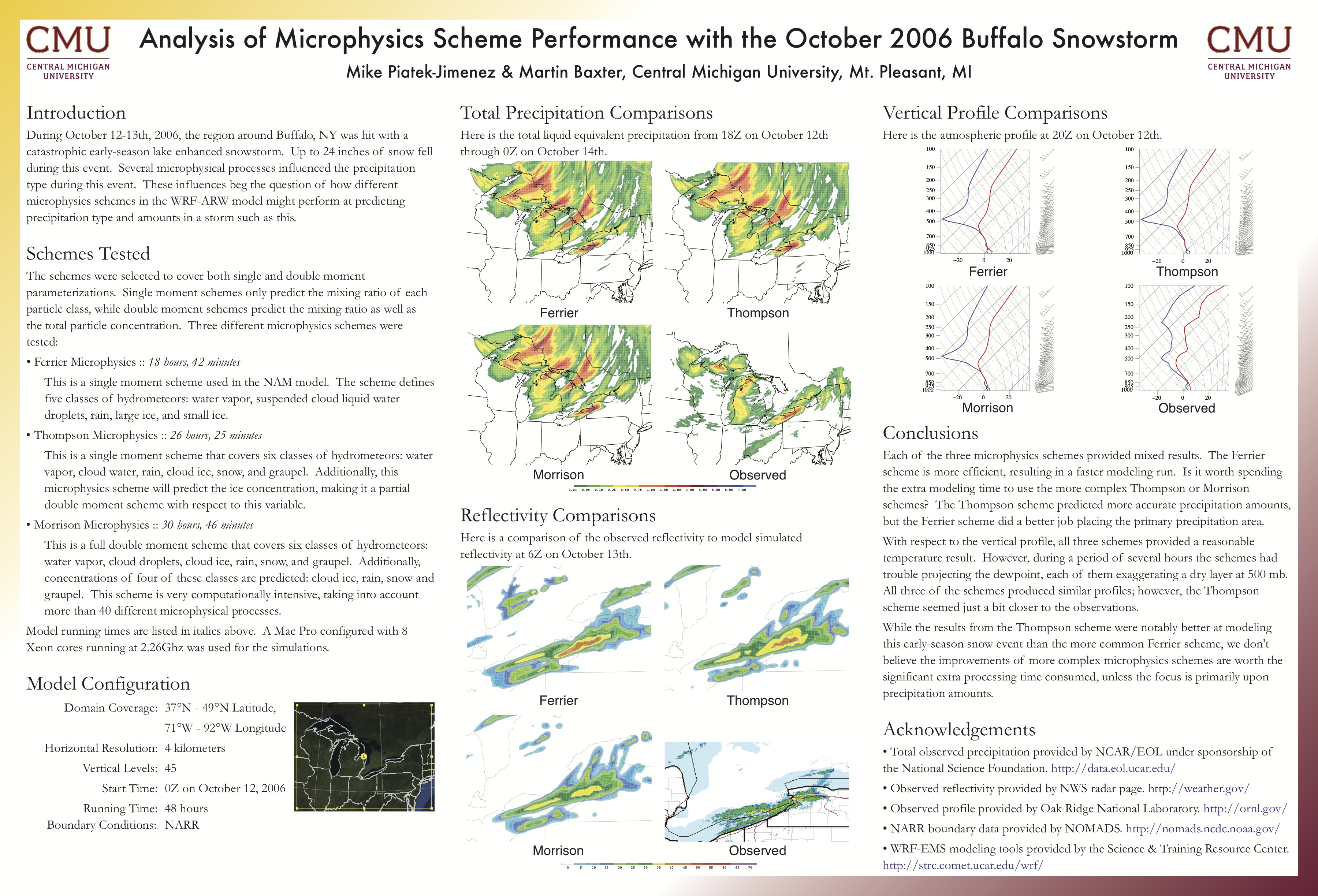
So it was easy for me to pick this storm (I even wrote about it back then). Next we (I’m working with my professor and friend, Marty, on this project) needed to pick something about the storm to focus upon. I can’t just put a bunch of pictures up and say, “Hey, look at all the snow!” There has to be some content. For this case study, Marty thought it might be interesting to look at how different microphysical schemes would effect a forecast over that time period.

This was a really tough event to forecast. Meteorologists could tell it was going to be bad, but with the temperature just on the rain/snow boundary, it was difficult to figure out just how bad it would be and where it would hit the hardest. If temperatures were a couple degrees warmer and this event resulted in rain instead of snow, it would have been a bad storm, but there wouldn’t have been the same devastation as there was with snow.

Microphysical schemes dictate how a forecast model transitions water between states. A microphysics scheme would determine what physical traits would have to be present in the environment to result in water vapor condensing to form liquid and create clouds, freeze into ice, or collide with other ice/water/vapor to form snowflakes. Some schemes take more properties of the atmosphere and physics into account than others, or weight variables differently when calculating these state changes. If I look at which scheme did the best job forecasting this event, then meteorologists could possibly run a small model with that same scheme on the next storm before it hits, to give them a better forecast tool.

To test these schemes, I have to run a model multiple times (once with each scheme). To do that, I had to get a model installed on my computer. Models take a long time to run (NOAA has a few supercomputers for this purpose). I don’t have a supercomputer, but my desktop Mac Pro (8×2.26 Ghz Xeons, 12 GB RAM) is a pretty hefty machine that might just let me run the model in a reasonable amount of time. I’m using the WRF-ARW model with EMS tools, which is commonly used to model synoptic scale events in academia. This model will compile on Mac OS X, but after a week of hacking away at it, I still didn’t have any luck. I decided to install Linux on the Mac and run it there. First I tried Ubuntu on the bare metal. It worked, but it was surprisingly slow. Next I tried installing CentOS in VMware Fusion, and it was actually faster (20%) than Ubuntu on the bare machine. The only explanation for this I can think of is that the libraries the model is compiled against were built using better compiler optimizations in the CentOS distribution. So not only do I get a faster model run, but I also can use Mac OS X in the background while it’s running. Perfect.

Once the model is installed, I have to setup a control run using parameters generally used in the most popular forecast models. There are several decisions that have to be made at this stage. First, a good model domain needs to be specified. My domain covers a swath 1720×1330 kilometers over most of the Great Lakes area, centered just west of Buffalo. For this large of a storm, a 4 km grid spacing is a pretty good compromise between showing enough detail and not taking years for the model to run. For comparison, the National Weather Service uses a 12 km grid spacing over the whole US to run their NAM forecast model 4 times a day. To complete the area selection, we have to decide on how many vertical levels to use in the model. Weather doesn’t just happen at the earth’s surface, and here I set the model to look at 45 levels from the surface up through around 50,000 feet. (I say “around” here because in meteorology we look at pressure levels, not height specifically, and with constantly changing pressure in the atmosphere the height can vary. The top surface boundary the model uses is 100 millibars.)

In case you didn’t notice, this kind of domain is quite large in computing terms. There is a total of 5,676,000 grid points in 3 dimensions. When the model is running, it increments through time at 22 second intervals. The model will calculate what happens at each of those grid points in that 22 seconds, and then it starts all over again. Usually, the model only writes out data after every hour, and I think it’s pretty apparent why this is the case. If I configured the model to output all the data at every time, there would be more than 44 billion point forecasts saved for the 2 day forecast run. Each of these forecasts would tell what the weather would be like at a particular location in the domain at a particular time, and each forecast would have around 30-50 variables (like temperature, wind speed, vorticity, etc). If those variables were simple 32 bit floats, the model would output about 6 TB of data (yes, with a T) for a single run. Obviously this is far from reasonable, so we’ll stick to outputting data every hour which results in a 520MB data file each hour. Even though we are outputting a lot less data, the computer still has to process the 6 TB (and the hundreds of equations that derive that data), which is quite incredible if you think about it.

My Mac is executing the control run as I’m writing this. To give you an idea, it will take about 12 hours for the model run to finish with VMware configured to use 8 cores (the model doesn’t run as quickly when you use hyperthreading) and 6 GB of RAM. This leaves all the hyperthreading cores and 6 GB of RAM for me to do stuff on the rest of my Mac, and so far I don’t notice much of a slowdown at all which is great.

So what’s next? Well after getting a good control run, I have to go back and test and run the model again for each of the microphysics schemes (there are 5-7 of them) and then look through the data to see how the forecast changes with each scheme. I’m hoping that one of them will obviously result in a forecast that is very close to what happened in real life. After I have some results, I will write up the content to fill a poster and take it with me to the conference at the beginning of October. The conference is in Tucson, which is great because I will have a chance to see some old friends while I’m there.

What does this mean for Seasonality users? Well, learning how to run this model could help me improve international Seasonality forecasts down the line. I could potentially select small areas around the globe to run more precise models once or twice a day. With the current forecast using 25-50km grid spacing, running a 12 km spacing would greatly improve forecast accuracy (bringing it much closer to the forecast accuracy shown at US locations). There are a lot of obstacles to overcome first. I would need to find a reasonably sized domain that wouldn’t bring down my server while running. Something that finishes in 2-3 hours might be reasonable to run each day in the early morning hours. This would be very long term, but it’s certainly something I would like to look into.

Overall it’s been a long process, but it’s been a lot of fun and I’m looking forward to not only sifting through the data, but actually attending my first meteorology conference a couple of months from now.